The way to use anthropometric data in the design process varies with the complexity of the problem.
Suppose you are designing a doorway to fit a population. You can measure everybody’s height and their body width across the arms. The whole population could then be accommodated by making the doorway tall enough for the tallest individual and wide enough for the widest individual. Costs can possibly be saved by deciding to accommodate only 90% of the population rather than all of the population. Reducing the size of the doorway to save money will require some people have to duck or turn sideways to get through.
Most design problems are considerably more complex than the doorway, however. Consider airplane cockpits, one-piece chemical protective suits, respirators or even office furniture. All of these require simultaneous consideration of many more than 2 dimensions to be effective. Research and experience have shown that using 5th and 95th percentile values for many dimensions results in considerably less than the desired accommodation (Robinette & McConville, 1981). Let’s look at why that is.
Suppose you want to accommodate 90% of a population for sitting height – a reasonable problem for the design of a car interior, for example. You would eliminate 5% of the tallest sitting heights and 5% of the smallest sitting heights leaving 90% accommodated in the center of the distribution.
Now, let’s suppose in your car you need to accommodate leg length so the driver can reach the pedals. You might take the central 90% of leg length as you took the central 90% of sitting height. But, the accommodation rate, instead of 90%, is actually 83% in a sample of males. Where did the other 7% go?
The reason for the drop in accommodation is that some of the 10% dropped for leg length are different people from the 10% dropped for sitting height. Because of this, the percent accommodated will decrease with each new dimension added. Further, to the extent that dimensions are not well correlated with each other – as hip breadth is not well correlated with sitting height – the decrease in accommodation will be even greater. To round out this example, if you added the central 90% of hip breadth to the sitting height and leg length requirements for your car, the total accommodated would drop to 78%. So with only 3 dimensions, instead of accommodating 90% of your population, you’re only taking care of just over three-quarters.
Now consider a more complex case – the aircraft cockpit – where there are a number of dimensions that are critical: the pilot needs to be able to see over the nose of the plane, reach the critical ejection handle, reach the foot controls, reach the joystick, reach the fuses overhead, but not be so tall as to hit the canopy with her helmet, and the knees can’t be so far forward that they are injured during an ejection. There are at least 12 important dimensions required to design that cockpit. It’s not possible to accommodate that many dimensions using a traditional percentile approach to capture the central 90% for each dimension.
So what’s the alternative?
One approach to complex problems like these is called multivariate accommodation modeling (MAM) and one approach to this sort of modeling is through principal component analysis (PCA). PCA is a computational technique that transforms a set of data into a set of new variables that are uncorrelated with each other. This is different from the original variables which have correlations among themselves. So in the cockpit example, you would use 12 input dimensions. The analysis would produce 12 new variables – the principal components (PC).
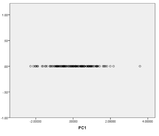
You can think about a single dimension – sitting height for example – as a line, and each person in your data set is a point on the line. There’s a minimum value, a maximum value, and everybody else is in between. A principal component has the same characteristic – everybody in the data set has a value for the principal component, and can be placed on the line (Figure 1). The difference is that the PC value is calculated from all 12 of the original values. The form of the calculation might be something like: sitting height * .234 + buttock-knee length * .193 + arm reach * .843 + … and so on to include all 12 original dimensions.

Figure 1. Sample data set along a single principle component (PC) line
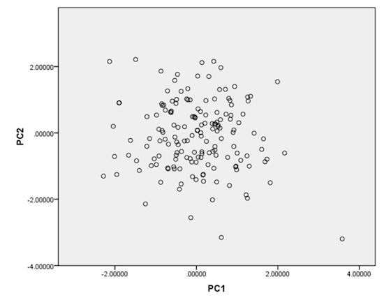
Now, the analysis is calculated in such a way that the first PC always contains as much of the total variance in the data set as possible. For anthropometric data sets, you can think of this as a general size PC. The second PC is calculated so it is orthogonal – at right angles – to the first PC. If you were to plot the two, PC1 and PC2 would be seen as two axes on a graph (Figure 2). The individual person’s would be dots scattered across the area.

Figure 2. Sample data set plotted with two PCs
PC2’s calculation has a similar form to the first PC (and to all PCs) in that it is a combination of all 12 original dimensions. It has the additional characteristic that it is completely uncorrelated with PC1. This means that all the variation accounted for by PC2 is different from variation accounted for by PC1. The third PC is orthogonal (at right angles) to the other two, so if you plotted it, it would form a 3-dimensional axis, and the dots would be arranged in 3 dimensions.
Because each PC is not correlated with the previous PCs, it turns out the variance in the data set is being organized much more efficiently. In fact, although there is always the same number of PCs as there are original dimensions, typically most of the data set variance is accounted for in the first 3 or 4 PCs. In this case, with 12 cockpit dimensions and a sample data set, the first 3 PCs account for 86% of all the variance in the population. The next 3 PCs account for less than 4% each, and the last 6 PCs account for less than 2% each. The happy news for your design problem is that instead of worrying about 12 dimensions for design, you can actually just worry about the first 3 PCs instead. Your design task has just become considerably easier.
So you’ve done your PCA, but how does that translate into a MAM that allows you to accommodate your intended audience?
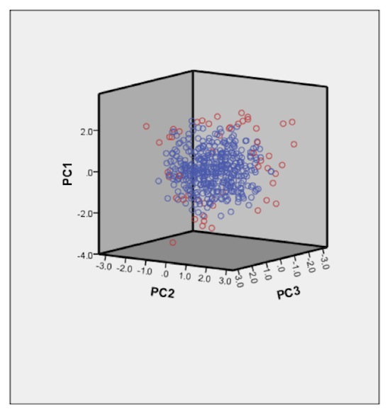
Figure 3 shows the data set graphed on the 3 PCs. Each of the circles represents a person in the data set. The blue circles represent the central 90% – the people you’re trying to accommodate. The individuals shown in red are the 10% outside the accommodation range. Notice that the circles are more densely situated in the center, and more sparsely towards the outside. This is a characteristic of a normal distribution – denser in the center, less dense towards the outside.
Remember also that these PCs are transformations of the original 12 dimensions. So, the people towards the center of the PC distribution are also closer to the center of the anthropometric distribution – and they are the people who are most ‘average’.
Now, there are no absolutely ‘average’ people, since we all vary from each other in some ways. But, those closer to the center of the distribution are more typical of the population as a whole, and those towards the outside are more unusual in some way. You take advantage of the distribution in moving from the PCA to MAM. Specifically, we will focus on designing for the periphery, with the idea that if you can accommodate those more unusual people on the edges, then the more average people near the center will be accommodated as well.

Figure 3. Sample data set distributed on 3 PCs (Blue = accommodated 90%; red = not accommodated 10%).
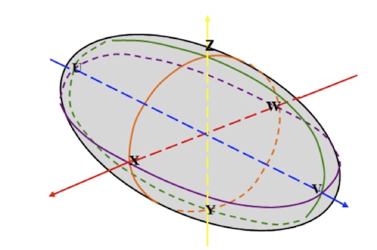
Figure 4 shows an accommodation ellipse. It’s a stylized form of the data in Figure 3. Basically, the ellipse was drawn around the central 90% of the population, and made into a smooth surface, but the characteristics are the same.
The people on the surface of the ellipse are more unusual, and the people near its center are more average.

Figure 4. 90% accommodation ellipse; data removed for clarity.
For design purposes, we are interested in the more unusual. Figure 4 has six specific points identified – U through Z, at the end of each of the three axes. There is no fixed number of design points that should be examined, but six should be a minimum. Many analysts use points between these six as well, for a total of 14, and some use two points between each axis point, for a total of 22. These points on the surface will become the multivariate accommodation models.
Whatever the number of models, the next step is the same. Recall that each of the PCs is a combination of the original 12 dimensions. Each of the surface points of interest is currently expressed as three coordinates. For example, the coordinates of Point Z might be PC1= 2.6, PC2 = 1.9, PC3 = 0.4. So you go back to the initial calculation of PCs, and identify the individual from the data set whose PC values are closest to point Z, and that person becomes your Point Z representative. You then pull out from the data set the original dimensions that produced the PC coordinates for your Point Z representative. This is repeated for all the models across the ellipse. When this is done, there is a collection of 6 or 14 or some other number of individuals – all unusual in at least one way – and you try to create your design to accommodate these individuals. The theory behind MAM is that if these individuals are accommodated, then the rest of the population on the interior will be accommodated as well.
This discussion wouldn’t be complete without some mention of some drawbacks associated with MAM and PCA.
First, this work requires access to raw data – that is, individual measurements for individual persons. It’s not possible to do it from published summary statistics of the population as a whole.
Second, I’ve presented a very high level discussion here to convey the general concepts. In practice there are a number of statistical considerations that may affect the outcome – for example whether to use original or normalized data, and whether to use a variance or a co-variance matrix in the calculation. Depending on the specific questions and the specific design goals, there will be different answers to these questions.
Third, PCA requires a multivariate normal distribution of the original data. Depending on the data set, and on the dimensions chosen, this assumption may not be met.
Fourth, the selection of dimensions for inclusion will affect the outcome, so considerable care needs to be given to this step.
Finally, if human testing – as opposed to computer modeling – is a part of the design process, it may be difficult to locate actual humans with these unusual anthropometric characteristics, since they are – by design – rare in the population. And in connection with this last, if your test design is shown to accommodate 5 of the 6 models, rather than all 6, it is not immediately possible to know what percentage of the population is disaccommodated. You know it is less than 90%, but you do not know how much less.
Those cautions aside, PCA-based MAM has proved useful in aircraft cockpit design (Hudson et al., 1998; Meindl et al., 1993), and has been thoughtfully proposed for use in respirator design, as well as the design of protective clothing, among other applications. Even with its difficulties, it almost always produces a more inclusive design than a reliance on univariate percentiles.
About the Author
Dr. Bruce Bradtmiller, president of Anthrotech, has 30 years experience in applied anthropometry. He was the contractor principal investigator for the recently completed Army’s ANSUR2 survey and for the original landmark ANSUR survey (1987-1988). He is an appointed expert to the International Standards Organization (ISO) technical committee on anthropometry, and is co-chair of the International Ergonomics Association (IEA) anthropometry technical group. He has received numerous prestigious awards including most recently the “Best Paper” award at the 9th International Congress of Physiological Anthropology, Delft, Netherlands. Anthrotech’s clients include government agencies and commercial firms both within the US and abroad. He can be reached at bruce@anthrotech.net, or 937-767-7226.
References
Hudson, J.A., G.F. Zehner and R.S. Meindl 1998 “The USAF Multivariate Accommodation Method”, Proceedings of the Human Factors and Ergonomics Society, 42nd Annual Meeting, Chicago, IL Human Factors and Ergonomics Society, Santa Monica, CA 90406.
Meindl, R.S., J.A. Hudson and G.F, Zehner 1993 A Multivariate Anthropometric Method for Crew Station Design, Armstrong Laboratory Technical Report AL-TR-1993-0054, Wright-Patterson Air Force Base, OH 45433.
Robinette, K.M., and J.T. McConville 1981 “An Alternative to Percentile Models”, SAE Technical Paper Series, Paper Number 810217, Society of Automotive Engineers, Warrendale, PA, 15096.
This article originally appeared in The Ergonomics Report™, with the title “Complex Anthropometry Made Simple”, on January 18, 2013. It is re-published here, with minor changes, by permission.
